From 500,000 Firewall Rules to an AI-Augmented Troubleshooter: What Actually Broke, and What Fixed It

A field report from building an AI pipeline on top of NSX-T, VRNI, and Neo4j — for infrastructure engineers who think
RAG and vector search are still buzzwords for someone else’s problem.

The Problem Nobody Warns You About

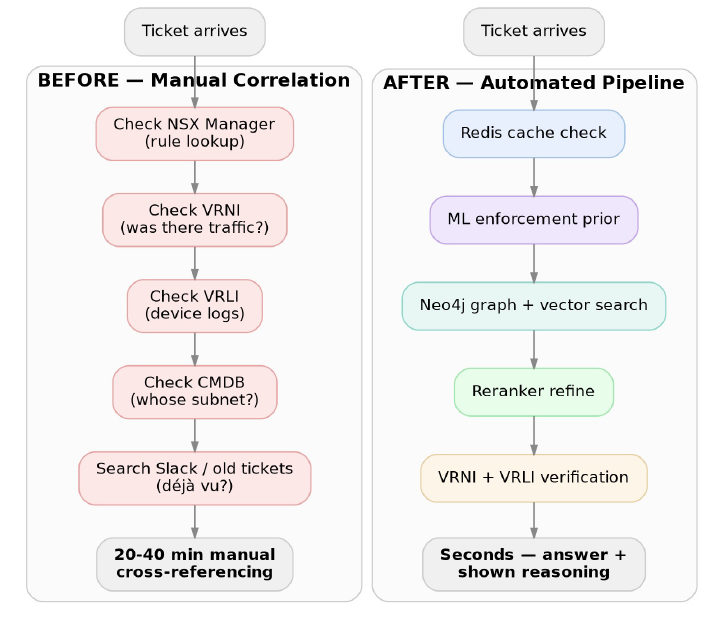
If you’ve run a firewall estate at any real scale, you know the drill. A ticket comes in: “traffic from 10.x.x.x to
10.y.y.y on port 443 is being dropped, please advise.” Somewhere in your environment there are 500,000+ FW
rules spread across multiple NSX-T managers, physical firewalls (Palo Alto, Fortinet, Check Point), and multi tenant
boundaries. The engineer’s job is to manually reconstruct: which subnet is the source in, which rule set applies, is
there a broader ALLOW being shadowed by a more specific DROP, has anyone actually seen this traffic pattern
before, and — critically — is this actually new, or did we see this exact thing three weeks ago and already fix it?

That last question is the one that quietly eats the most time. Institutional knowledge about “we’ve seen this before”
lives in people’s heads, old ticket comments, and Slack threads — not in a queryable form. This post is about the
pipeline I built to fix that, the specific technical dead ends I hit along the way, and the reasoning behind every tool I
picked (and didn’t pick).

Issue #1: A Graph Database Alone Doesn’t Understand Meaning

The setup. I’d already connected CMDB, RVTools (VM inventory), VRNI (network flow logs), IPAM, and DFW rules
into a Neo4j graph. This is genuinely powerful for anything with an explicit, known structure: VM → subnet → rule →
firewall → tenant, all walkable in one Cypher query. CIDR containment, rule priority checks, root-cause path-finding
— a graph is the correct data model for this, full stop.

Where it broke down. Two rules can be functionally identical — same intent, same effective traffic pattern — but
written years apart by different engineers, with different comment wording, different CIDR granularity, or a slightly
different port range that happens to cover the same real traffic. A pure Cypher WHERE clause matching on exact
properties will never surface that these two rules are “basically the same thing.” Neo4j knows relationships; it
doesn’t know meaning.

Rule A: “Allow web tier to DB tier, prod” src: 10.10.4.0/24 dst: 10.10.8.10/32 port: 5432
Rule B: “App servers to Postgres primary” src: 10.10.4.0/25 dst: 10.10.8.10/32 port: 5432

Same intent, overlapping but not identical CIDRs, completely different description text. Exact-match search finds
neither as a duplicate of the other.

The fix: embeddings. I’m already running bge-m3 on my own inference platform (via LiteLLM) — an embedding
model that converts text into a vector representing its meaning, not its literal characters. Rule descriptions, ticket
text, and incident notes get embedded once, and Neo4j’s native vector index (available since 5.x — no separate
vector database needed) lets you query by semantic similarity in the same graph, on the same nodes, alongside
your existing relationship traversal.

CALL db.index.vector.queryNodes(‘rule_embeddings’, 20, $query_vector)
YIELD node AS rule, score AS vector_score
MATCH (rule)-[:APPLIES_TO]->(subnet:Subnet)
WHERE subnet.tenant = $tenant
RETURN rule.id, rule.description, vector_score
ORDER BY vector_score DESC LIMIT 20

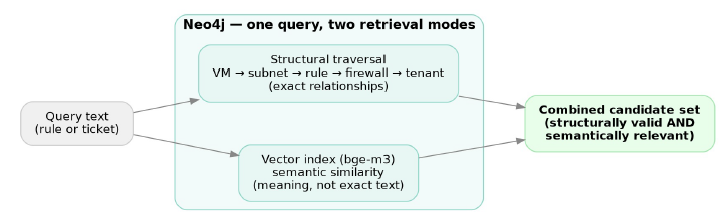
Neo4j combining structural graph traversal with semantic vector search in one query

One query, two retrieval modes — structural graph traversal and semantic vector similarity, at once. This is the
pattern generally called GraphRAG, and it’s the single highest-leverage change in this whole pipeline.

Issue #2: Vector Search Alone Is Noisy

The setup. Once vector search was live, it worked — but “worked” meant returning a top-20 list where maybe 8
were genuinely relevant and 12 were semantically-adjacent-but-wrong. Vector similarity measures overall closeness
in meaning space; it doesn’t do the deeper, more expensive read of “does this document actually answer this
specific query.”

The fix: a reranker. gte-reranker , also served on the same inference platform, takes the user’s actual query text
and each candidate document as a pair, and does a full cross-attention pass to score true relevance — far more
accurate than vector similarity, but too computationally expensive to run against all 37,000 rules directly. The
pattern: vector search narrows 37,000 → ~20 (cheap), reranker refines 20 → top 5 (accurate but only run on the
small shortlist).

Vector search narrows to 20 candidates, then the reranker refines to the top 5

This two-stage retrieval — cheap-and-broad, then expensive-and-narrow — is standard in production RAG systems
for exactly this reason: neither stage alone gets you both speed and accuracy.

Issue #3: Every Query Hitting the LLM Gets Expensive, Fast

The setup. Once the LLM (in my case GLM-5.2 or Qwen-based models, tiered by task) was generating the final
diagnosis, every single query — including ones that were near-duplicates of something asked an hour earlier —
triggered a full model call. At troubleshooting-tool scale, with multiple engineers asking variations of the same
handful of recurring issues, that’s a lot of redundant GPU time.

The fix: Redis as a cache layer — in front of everything, not just the LLM. Redis isn’t a database
replacement for Neo4j; it’s a fast, ephemeral, key-value cache that sits in front of both the LLM calls and the
reranker calls.

Deployment: standalone RHEL VM
maxmemory-policy: allkeys-lru ← critical: evict oldest, never crash on full memory
persistence: light RDB, no AOF ← everything here is regenerable from source of truth
ACLs per consumer (LiteLLM, DFW Checker, Jarvis) instead of one shared password

Two cache layers, specifically: 1. LLM response cache (exact-match and semantic near-duplicate) — LiteLLM
supports this natively 2. Reranker result cache, keyed on (query_text, candidate_id_set) — skips the expensive
cross-attention pass entirely on repeat queries

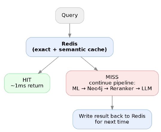
Redis cache hit returns instantly; a miss falls through to the rest of the pipeline and writes back

Issue #4: A Cache That Doesn’t Know When It’s Wrong Is Worse Than No
Cache

The setup. This is the trap that’s easy to miss until it bites you. A cached “why is this dropping” answer is only
correct until someone pushes a rule change affecting that exact traffic. TTL-based expiry (just wait N minutes and
hope) means you’re either serving stale, actively wrong answers for a while, or setting TTLs so short the cache
barely helps.

The fix: tie invalidation to the event you already have. Every firewall rule push in my environment already
syncs to Neo4j — that’s an existing trigger, not new plumbing. The fix was making that same sync event also invalidate exactly the Redis keys derived from the changed rule, using a tagging index rather than a guess

#At cache-write time
redis.set(cache_key, result, ex=ttl)
redis.sadd(f”rule:{rule_id}:cache_keys”, cache_key)
#On rule-change sync event (existing hook)
def on_rule_change(rule_id):
keys = redis.smembers(f”rule:{rule_id}:cache_keys”)
if keys:
redis.delete(*keys)
redis.delete(f”rule:{rule_id}:cache_keys”)

This turns the cache from “stale until timeout” into “correct immediately after any relevant change” — the
difference between a cache that saves time and one that quietly erodes trust in the tool.

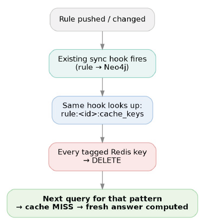
Rule change triggers targeted Redis key invalidation via the existing Neo4j sync hook

Issue #5: The Temptation to Reach for a Neural Network When You Don’t
Need One

The setup. Once you’re deep in embeddings, rerankers, and LLMs, everything starts to look like a deep-learning
problem. I hit this directly when building an ALLOW/DROP enforcement predictor: given a historical flow tuple
(source, destination, port, protocol), predict whether it gets dropped, using millions of rows of past VRNI flow
outcomes.

The fix: match model complexity to data shape, not to what’s trendy. Four input features, tabular, with a
clear historical base-rate signal — that’s the textbook case for logistic regression or gradient boosting (XGBoost),
not a neural network. A neural net needs volume and dimensionality to justify its complexity; with this little
structure, a tree-based model matches or beats it on accuracy, trains in seconds on CPU, and — critically for a
troubleshooting tool — stays interpretable: you can see which feature drove a prediction, not just the number.

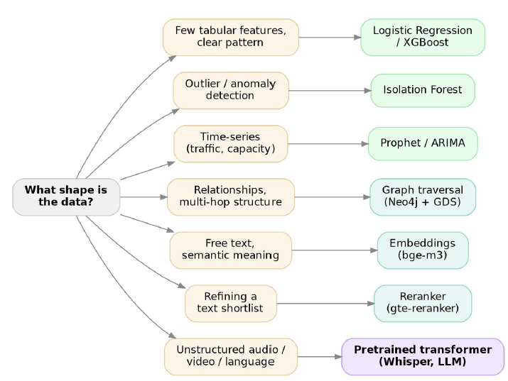
Decision tree: matching data shape to the right modeling tool

Neural networks earned their place exactly once in this stack: a separate call-intelligence project turning audio into
structured meaning, where the input is genuinely unstructured. Everywhere else — tabular flow data, graph
relationships — a neural net would have been the wrong tool wearing a trendy hat.

This model runs as the first check in the troubleshooting pipeline, before anything touches the graph, precisely
because it’s the cheapest signal available: milliseconds, no database round-trip, subnet index baked into a selfcontained
pickle file.

Issue #6: A Rule Match Isn’t Proof — You Have to Verify Against What
Actually Happened

The setup. Everything above — the graph, the vectors, the reranker, the ML prior — produces a hypothesis:
“based on rule structure and history, this traffic should behave like X.” That’s not the same as knowing what
actually happened on the wire. Rules describe intent. They don’t guarantee reality. A rule can look correct in the
NSX manager and still not be why traffic is failing — routing, a host-based firewall, an intermediate hop, or simple
rule-priority ordering can all produce a mismatch between “what the rule says” and “what the packet actually did.”

The fix: cross-check the hypothesis against two independent sources of ground truth before trusting a
diagnosis.
VRNI (flow-level truth) — did the traffic actually flow at all, in either direction, at what volume, and when? If
the rule chain says ALLOW but VRNI shows zero flows in either direction, the problem likely isn’t the firewall
rule — it’s routing, or the destination service isn’t listening, or the source never actually attempted the
connection.
VRLI (log-level truth) — what did the enforcement device itself log? This is the actual accept/deny event
from NSX-T or the physical firewall, correlated by timestamp and tuple. If VRLI shows an explicit DENY logged
by the device even though the rule you found in the graph says ALLOW, that’s a strong signal of a rule-priority
conflict — a more specific DROP rule higher in evaluation order is shadowing the ALLOW you matched on.

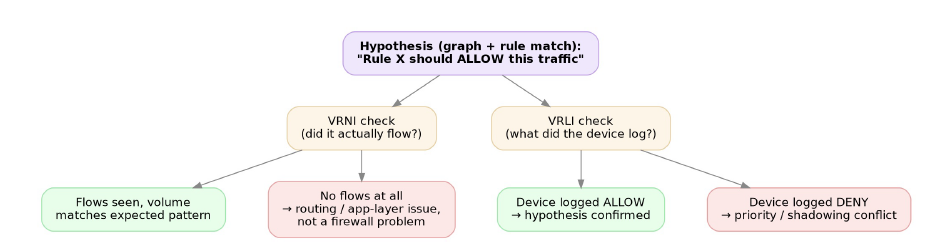
Ground-truth verification: cross-checking the rule hypothesis against VRNI flow data and VRLI device logs

The other checks that guard against a false diagnosis before it ever reaches VRLI/VRNI: – CIDR-aware
rule matching — confirming the resolved subnet actually falls inside the rule’s declared scope, not just a loose IPstring
match – ALLOW vs. DROP priority ordering — checking evaluation order explicitly, since NSX-T (like most
firewalls) evaluates top-down and a broad ALLOW lower in the list never overrides a narrower DROP above it –

CMDB/IPAM consistency — confirming the resolved owner, tenant, and subnet classification actually agree across
sources before trusting the graph relationship at all; a stale CMDB record pointing to the wrong tenant would
silently poison every downstream check
Only once the rule-based hypothesis, the priority check, and both independent log/flow sources agree does the
pipeline hand a confirmed diagnosis to the LLM to narrate — rather than the LLM confidently explaining something
that was only ever a plausible-looking rule match. This is the difference between an AI tool that sounds right and
one that’s actually checked its own answer against reality before saying anything.

The Full Pipeline, End to End

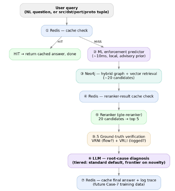
Full end-to-end pipeline: Redis, ML predictor, Neo4j hybrid retrieval, reranker, VRNI/VRLI verification,
tiered LLM, and cache write-back

Cost and latency stack cheapest-first: a Redis lookup costs ~1ms, ML inference ~10ms, the graph+vector query
~50-100ms, the reranker ~200-500ms, and the LLM call is the expensive tail end — seconds, especially on frontiertier
models. Most repeated or routine questions resolve in the first two stages and never reach the LLM at all.

Why Each Product, Specifically

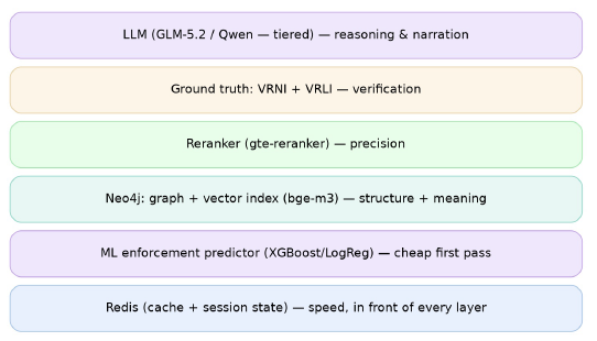
Layered stack: Redis and the ML predictor sit as cheap early layers, Neo4j and the reranker in the
middle, ground truth and the LLM at the top

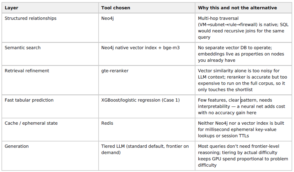
What I’d Tell Someone Starting This From Scratch
Build in the order the cost curve suggests, not the order that feels most “AI”:

1. Redis first — it’s foundational infrastructure everything else will lean on, and the LLM cache alone pays for
   the effort almost immediately.
2. Vector index on your existing graph — you already have the data; embedding it and adding a vector
   index is additive, not a rebuild.
3. Reranker — only once retrieval is noisy enough to notice; don’t add it prematurely.
4. Cache invalidation tied to your real change events — do this before you trust the cache in production,
   not after a stale answer causes an incident.
5. Classical ML for tabular signals — resist the urge to reach for a neural network until your data actually
   stops being tabular.

The unifying lesson across every one of these decisions: the right tool is determined by the shape of the data and
the cost of being wrong or slow — not by which tool is newest. A graph for relationships, embeddings for meaning, a
reranker for precision, a cache for speed, classical ML for structured tabular signals, and a neural network only
when the input is genuinely unstructured. Once that framework clicks, the specific product names become
swappable details.