Building the Backend: AI Fabric Design from Scalable Units to Lossless RoCEv2

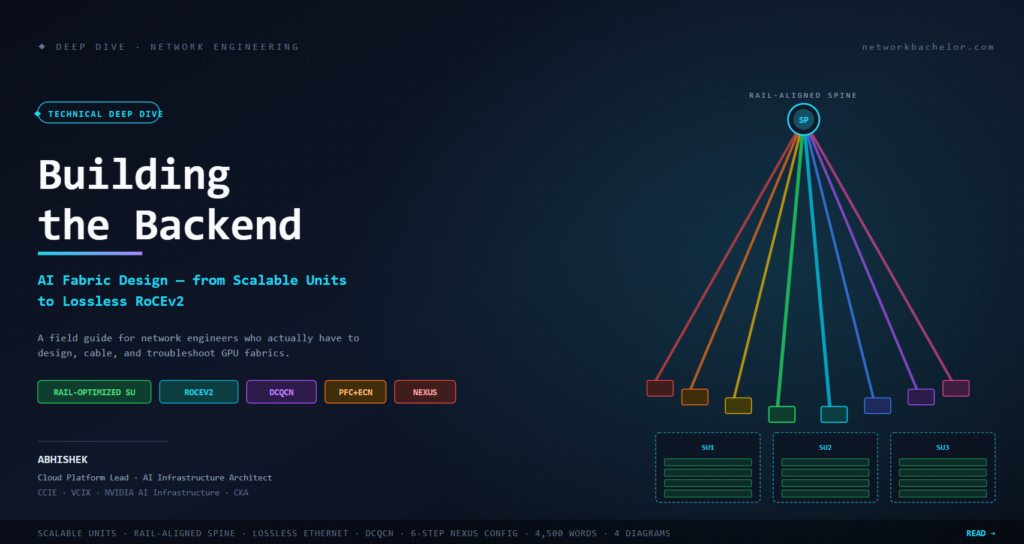
A network engineer’s field guide to the physics, topology, and QoS discipline behind modern GPU clusters — with Nexus config that actually runs.

---

0. Why This Post Exists

Almost every “AI networking” article on the internet stops at “you need low latency and high bandwidth.” That is the equivalent of telling a CCIE candidate that BGP is “a routing protocol.” Useful for a LinkedIn headline, useless in a rack.

This post is written for the network engineer who has to actually design, cable, configure, and troubleshoot a GPU fabric. We will cover:

1. Why AI workloads break traditional DC assumptions — the collective communication problem
2. The Scalable Unit (SU) — the atomic building block of modern GPU DCs
3. Rail-optimized leaf-spine — why the spine sometimes carries zero traffic
4. Physical rack design — power, cooling, and the 256-fiber structured-cabling problem
5. Transport layer — InfiniBand vs RoCEv2, decided on merits, not marketing
6. Lossless Ethernet mechanics — PFC, ECN, DCQCN, and the CNP feedback loop
7. Nexus config walkthrough — a two-switch RoCEv2 lab that mirrors production
8. Verification, counters, and the failure modes nobody warns you about

No fluff. If a section doesn’t teach you something you can use on Monday, it doesn’t belong here.

---

1. Why AI Workloads Break Traditional DC Networking

Traditional enterprise east-west traffic is bursty, asymmetric, and small-flow-heavy. A web tier hits an app tier hits a DB tier. TCP handles reordering and loss. A dropped packet costs a retransmit — a few RTTs, no user notices.

GPU training is nothing like that. A single training step for a large model looks like this:

compute (forward pass)  -->  compute (backward pass)  -->  AllReduce across N GPUs  -->  next step

That AllReduce is a synchronous collective. Every GPU in the ring/tree waits for every other GPU. If one flow is 5 µs slower than the others, the entire cluster stalls for 5 µs on every iteration. Multiply by billions of iterations. The tail latency of the slowest packet becomes the effective performance of the fabric.

Three consequences fall out:

• Loss is catastrophic. RDMA (the transport underneath NCCL) uses go-back-N or selective repeat. A single dropped packet stalls the connection for tens of microseconds — an eternity when your step time is measured in milliseconds.
• Jitter is the enemy. Even without loss, variance between rail latencies destroys collective performance. You are designing for P99.99, not average.
• Flows are elephant, symmetric, and predictable. A GPU-to-GPU transfer is a multi-GB blast that saturates a 400G link. ECMP flow hashing based on 5-tuple works — but only if you engineer the entropy correctly and avoid hash polarization.

The takeaway: you are not building a data center network. You are building a compute fabric where the network is part of the memory hierarchy. The design discipline is closer to HPC than to enterprise DC.

---

2. The Scalable Unit (SU): The Atomic Building Block

The reference architecture that has emerged across NVIDIA DGX SuperPOD, Meta’s RSC, and every hyperscaler’s internal design is the Scalable Unit (SU).

An SU is a self-contained power, cooling, and networking domain. It is sized so that you can deploy one, validate it, and then buy N more without re-architecting anything.

The typical SU dimensions (DGX H100/H200-class)

Property	Value	Why
GPUs per node	8	DGX H100/H200 chassis standard
Back-end NICs per node	8 (one per GPU, called a rail)	Rail-optimized topology
Nodes per compute rack	4	Power/cooling ceiling (~10–12 kW per node)
Compute racks per SU	8	4 × 8 = 32 nodes
Total nodes per SU	32	Fits one leaf switch’s port budget
Leaf switches per SU	8 (one per rail)	32 downlinks × 8 rails
Network racks per SU	1 (dedicated, holds all 8 leaves)	Structured cabling, not adjacency
Total back-end NICs	256 (32 nodes × 8 rails)	This is the fiber count into the net rack

The concept that trips people up: leaf switches do not live in compute racks

This is the single most common misconception when a network engineer transitions into AI infrastructure. In a traditional Top-of-Rack (ToR) design, each compute rack has its own leaf switch at the top. Cabling is short, contained, and rack-local.

AI fabrics abandon ToR entirely for the back-end.

Instead, all 8 leaf switches for an SU live together in a dedicated network rack. Every server’s rail-0 NIC — regardless of which compute rack it sits in — is cabled to a single leaf switch (call it Leaf-0). Every rail-1 NIC across all 8 compute racks goes to Leaf-1. And so on.

Why? Two reasons:

1. Port density. A modern 64-port 400G leaf can serve 32 downlinks (one per node in the SU) using only half its faceplate. Splitting that across 8 racks with partial-populated leaves wastes ports, wastes power, and multiplies switch count 8× for no benefit.
2. Rail isolation. Keeping every rail on its own physical switch means intra-rail collective traffic never crosses a rail boundary. The NCCL topology can align with the physical topology, and the ring/tree algorithms achieve their theoretical bandwidth.

The cost is structured cabling. You are pulling 256 fibers from 8 compute racks into 1 network rack. That is a real physical-plant engineering exercise — MPO-24 trunk cables, patch panels, cable trays sized correctly. This is where “network engineer” starts to overlap with “facilities engineer.”

The niche diagram: rail-optimized SU layout

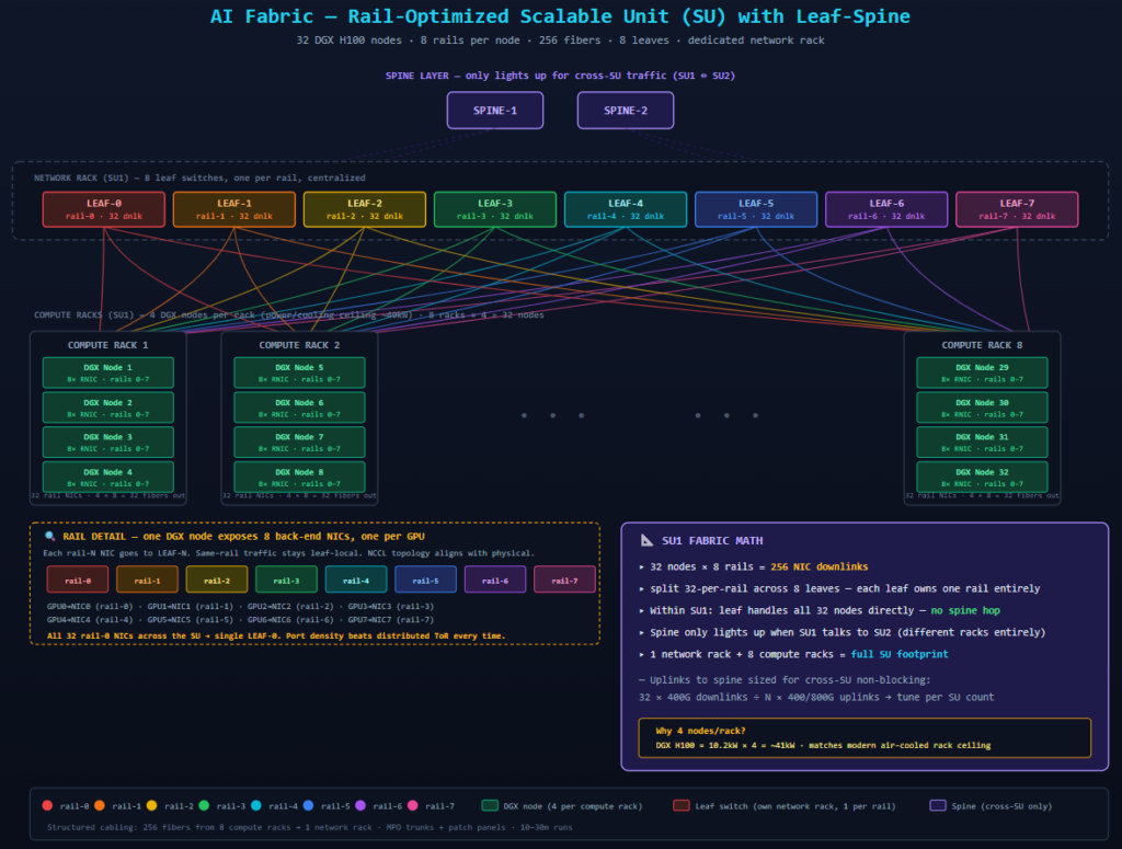
The fabric math

Within a single SU, every leaf handles all 32 nodes for its rail directly. No spine hop is required. This means:

• Intra-SU rail-N to rail-N traffic = 1 leaf hop (server → leaf → server)
• Intra-SU cross-rail traffic = never happens in NCCL rings; the topology avoids it
• Cross-SU traffic = 3 hops (leaf → spine → leaf on the far SU)

The spine layer is provisioned only when you deploy 2+ SUs. A single-SU deployment can defer spine investment entirely — a real capex win for early-stage clusters.

The spine layer is provisioned only when you deploy 2+ SUs. A single-SU deployment can defer spine investment entirely — a real capex win for early-stage clusters.

Scaling to N SUs: the rail-aligned spine plane

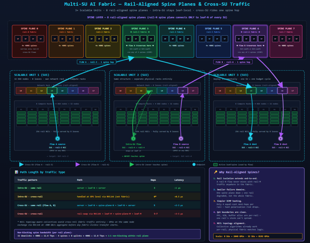
The moment you deploy a second SU, the spine has to actually carry traffic. But how you build the spine determines whether your fabric behaves gracefully at scale or turns into an operational nightmare.

Two schools of thought:

Traditional (shared) spine. All 8 leaves in every SU uplink to a common pool of spine switches. Every spine is reachable from every rail. Simple to draw on a whiteboard. But it destroys rail isolation: a rail-3 flow and a rail-6 flow can now hash to the same spine ECMP path, share buffers, and interfere with each other. A PFC storm on rail-2 can propagate into rail-5’s queues on a shared spine.

Rail-aligned spine planes. This is what NVIDIA SuperPOD-class designs actually deploy. You build N independent spine planes, one per rail. Spine plane 3 has connectivity only to Leaf-3 of every SU. Spine plane 6 has connectivity only to Leaf-6 of every SU. There are effectively 8 parallel, non-interfering fabrics stacked on top of each other.

The consequences are large:

• Rail isolation extends end-to-end. Whatever isolation you got by putting rail-3 traffic on Leaf-3 continues all the way to the spine. Rail-6 traffic never touches rail-3’s switches, buffers, or ECMP paths — anywhere.
• Smaller failure domains. If a spine goes down, only one rail loses redundancy. NCCL degrades gracefully because seven other rails are still full-speed.
• Simpler ECMP. Each leaf has to hash across only ~4 spine next-hops within its plane, not across all spines in a shared pool. Hash polarization is less likely, and when it happens it affects one rail, not the fabric.
• QoS boundaries are clean. PFC, ECN thresholds, buffer allocation, and priority queues can be tuned per rail plane, or even differently per plane, without cross-contamination.

The path length table

Once you have multiple SUs and rail-aligned spines, the fabric path length depends entirely on the source-destination pair:

Traffic pattern	Path	Hops	Latency (typical)
Intra-SU · same rail	server → leaf-N → server	3	~1 µs
Intra-SU · cross-rail	GPU-to-GPU via NVLink (not fabric)	0*	~0.5 µs
Cross-SU · same rail	server → leaf-N → spine-plane-N → leaf-N → server	5	~2–3 µs
Cross-SU · cross-rail	rail-swap via NVLink → leaf-M → spine-plane-M → leaf-M	5–7	~3–5 µs

* NCCL’s topology-aware collectives avoid cross-rail fabric traffic entirely on a single node — GPU-to-GPU exchanges happen on NVLink at ~900 GB/s aggregate before any fabric-visible transfer starts. The fabric only sees rail-N to rail-N flows.

Bandwidth math for the spine plane

Non-blocking design for one rail plane serving M SUs:

Per-plane downlinks (from all SUs)   =  M SUs × 32 leaf downlinks × 400G
Per-plane uplinks (leaf → spine)      =  M SUs × N_uplinks × 400G

For non-blocking: N_uplinks × 400G ≥ 32 × 400G per leaf
                → N_uplinks ≥ 32 per leaf (or half that at 800G)

For an 8-SU deployment with 400G rails, you need roughly 4 spines per rail plane and 32 spine-facing ports per leaf. That’s 8 planes × 4 spines = 32 spines total to serve 2048 GPUs non-blocking. Above that scale, you introduce a super-spine tier or accept controlled oversubscription — 2:1 is common, 4:1 pushes NCCL performance for very large collectives.

---

3. Physical Rack Design: The Constraints You Can’t Refactor

Software problems have workarounds. Physical constraints do not.

Power

A DGX H100 draws roughly 10.2 kW at full tilt. H200 and B200 are higher. Facility rack budgets vary wildly:

Facility tier	Typical rack ceiling
Legacy colo	6–8 kW
Standard modern DC	15–25 kW
AI-ready DC (air)	30–40 kW
AI-ready DC (DLC)	60–120 kW+

At 10 kW per node, an air-cooled 40 kW rack fits 4 nodes. That is not a coincidence — it is the constraint the entire SU dimensioning is built around. If you have direct liquid cooling (DLC), you can stack 8+ nodes per rack, and the SU math shifts.

Cooling

Nodes exhaust hot air at the back at ~40°C+. Hot aisle containment is mandatory. Rear-door heat exchangers or immersion baths become necessary above ~30 kW/rack. This is not a networking topic until it forces your rack unit count down, which forces your rack count up, which forces your cable runs longer, which forces your optics choice.

Cabling

For a 32-node SU:

• Back-end (rail) fibers: 32 nodes × 8 rails = 256 fibers from compute racks to network rack. At 400G, these are OSFP or QSFP112 with duplex LC or MPO connectors. Runs are typically 10–30 m.
• Front-end (management/storage): additional 2–4 NICs per node for storage and in-band management. Different fabric, usually still Ethernet.
• Inter-switch (leaf-to-spine): N × 400G or 800G per leaf, depending on oversubscription target. Non-blocking designs demand equal aggregate uplink capacity to server-facing capacity.

Pull the wrong fiber type once and you are re-cabling a live rack while someone’s training run bleeds money. Structured cabling with pre-terminated MPO trunks and patch panels at both ends is not optional at this scale.

---

4. Transport Layer: InfiniBand vs RoCEv2

This is the religious war of AI networking. Let’s dispense with the religion and look at the mechanics.

InfiniBand at a glance

InfiniBand is a lossless, credit-based transport designed from day one for RDMA. Key properties:

• Credit-based flow control (link layer). A sender may only transmit if the receiver has advertised credits. No credits, no send. This makes IB natively lossless — there is no equivalent of a switch buffer overrun causing a drop.
• Subnet Manager (SM). A centralized controller programs LFTs (Linear Forwarding Tables) on every switch. Adaptive routing decisions are computed globally.
• Adaptive Routing (AR). Switches can hash flows across multiple equal-cost paths in hardware, and reroute around congestion in real time.
• SHARP (Scalable Hierarchical Aggregation and Reduction Protocol). In-network reduction — the switch itself performs the AllReduce arithmetic, halving the traffic on the fabric.
• NDR generation: 400 Gb/s per port; XDR at 800 Gb/s.

The tradeoff: single-vendor (NVIDIA/Mellanox), higher $/port, and your ops team needs IB-specific tooling (ibnetdiscover, iblinkinfo, perfquery). If your team is Ethernet-native, you are paying an operational tax.

RoCEv2 at a glance

RoCEv2 (RDMA over Converged Ethernet v2) is RDMA transport packaged inside a UDP/IP packet, running on standard Ethernet:

Ethernet header │ IP header │ UDP header (dport 4791) │ IB BTH │ RDMA payload │ ICRC

Key properties:

• UDP encapsulation allows standard 5-tuple ECMP hashing on Ethernet fabrics. Src port is randomized per QP (queue pair) to spread entropy.
• No native flow control. Ethernet is lossy by default. RoCEv2 requires you to engineer the underlay to behave losslessly — this is where PFC and ECN come in (Section 5).
• DCQCN (Data Center Quantized Congestion Notification) is the ECN-driven end-to-end congestion control algorithm implemented in RNIC hardware.
• Multi-vendor. Any Ethernet switch that supports lossless queuing (Nexus 9300/9500, Arista 7060/7280, Cisco 8000, Juniper QFX/PTX) can carry RoCEv2.
• 400G/800G standard on modern silicon (Broadcom Tomahawk 4/5, Cisco Silicon One).

The tradeoff: you inherit all of Ethernet’s flexibility and all of its complexity. QoS misconfiguration silently degrades performance. There is no SM to catch your mistakes.

The honest comparison

Dimension	InfiniBand	RoCEv2
Loss behavior	Natively lossless	Engineered lossless (PFC/ECN)
Congestion control	Credit-based + AR	DCQCN (ECN + hardware rate limit)
Routing	SM-managed, adaptive	ECMP, sometimes DLB
In-network reduction	SHARP	None (roadmap: SwitchML, NCCL-IN)
Ops tooling	IB-specific	Standard Ethernet
Vendor diversity	Single (NVIDIA)	Multi-vendor
$/port	Higher	Lower
Ecosystem maturity for AI	Very mature	Rapidly maturing
Fault domain isolation	Excellent	Depends on config

Both work. Both are shipping in hyperscale AI DCs today. The decision is more about your team, your existing infrastructure, and your vendor strategy than about technology.

The rest of this post focuses on RoCEv2, because that’s where the QoS engineering conversation actually lives — IB handles most of this for you.

---

5. Lossless Ethernet: PFC, ECN, and the DCQCN Feedback Loop

To make RoCEv2 work, the Ethernet underlay must guarantee zero packet loss for the RDMA class. Ethernet is not lossless by default. We build it up in two layers.

Layer 1: PFC (802.1Qbb) — the emergency brake

Priority Flow Control is a hop-by-hop link-layer pause mechanism. When a switch’s ingress queue for a specific priority hits a threshold, it sends a PAUSE frame to the upstream device. The upstream stops sending traffic for that priority only, for a specified duration.

Critical properties:

• Per-priority. Only the RoCEv2 class pauses. Other traffic on the link keeps flowing.
• Hop-by-hop. PFC does not signal end-to-end. It builds up backwards, hop by hop, from the congestion point toward the source.
• Buffer headroom required. When you send a PAUSE, in-flight frames are already on the wire. The receiver must have buffer to absorb them. This is why jumbo MTU (9216) is standard for RoCE — bigger frames × cable length × link speed = required headroom.
• PFC storms are real. A misconfigured or stuck receiver can PAUSE indefinitely, black-holing the entire link. This is what the PFC watchdog (priority-flow-control watch-dog-interval on) is for — it detects a stuck queue and forces it to drain.

PFC is the last line of defense. If you rely on PFC as your primary congestion control, you have already lost — the fabric is oscillating between paused and unpaused, and throughput craters.

Layer 2: ECN + DCQCN — the proactive rate limiter

The right way to control congestion is to slow the sender before the queue fills. That’s what ECN + DCQCN does.

Explicit Congestion Notification (ECN) is two bits in the IP header:

• 00 — Non-ECT (Not ECN Capable Transport)
• 10 / 01 — ECT (ECN-Capable Transport)
• 11 — CE (Congestion Experienced)

The DCQCN loop works like this:

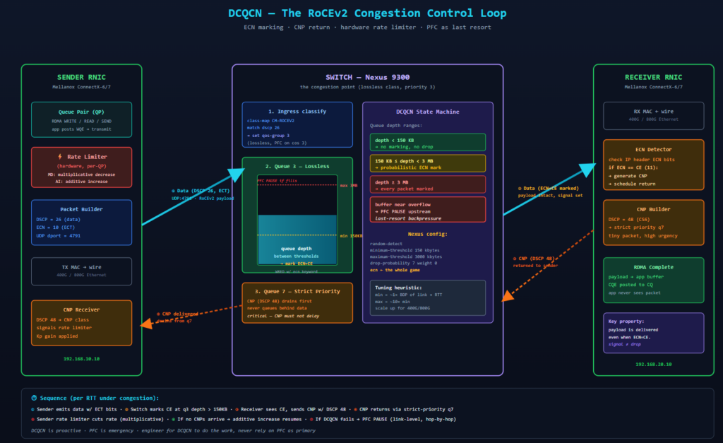
The critical detail: the Congestion Notification Packet (CNP) must never be dropped or delayed. If the CNP gets stuck in a congested queue, the sender never learns to slow down, and the queue keeps growing until PFC kicks in. This is why we put CNP in its own strict-priority queue (QoS group 7) with a different DSCP marking (DSCP 48 / CS6).

DCQCN parameters you control at the switch:

• Minimum threshold — queue depth below which no marking occurs
• Maximum threshold — queue depth at which every packet is marked
• Drop probability — the slope of the marking probability curve between min and max
• Weight — the WRED averaging weight (0 = instantaneous)

The lab in the next section uses:

random-detect minimum-threshold 150 kbytes
              maximum-threshold 3000 kbytes
              drop-probability 7 weight 0 ecn

These are reasonable starting values for a 100G link. You will need to tune them for your specific link speed, RTT, and workload. The general principle: mark early enough that DCQCN reacts before PFC has to.

---

6. Nexus Config Walkthrough: A Runnable Two-Switch RoCEv2 Lab

The following is a working, minimum-viable RoCEv2 config for a pair of Nexus 9300 switches in a leaf-leaf topology. This is the config from the reference diagram, annotated. Deploy it identically on both switches unless noted.

Topology recap

   Server 1 ──────── Nexus-Leaf-1 ─────100G─────  Nexus-Leaf-2 ──────── Server 2
   192.168.10.10    Eth1/1     Eth1/49        Eth1/49      Eth1/1     192.168.20.10
                    (192.168.10.0/24)                                 (192.168.20.0/24)
                                    L3 routed: 10.255.0.0/31

Step 1 — Classification (ingress DSCP → QoS group)

class-map type qos match-any CM-ROCEV2
  match dscp 26

class-map type qos match-any CM-CNP
  match dscp 48

policy-map type qos PM-QOS-ROCE-INPUT
  class CM-ROCEV2
    set qos-group 3
  class CM-CNP
    set qos-group 7
  class class-default
    set qos-group 0

What it does: any packet arriving with DSCP 26 (RoCEv2 data) is placed in QoS group 3. DSCP 48 (CNP) goes to group 7. Everything else lands in the default group 0.

Why DSCP 26 and 48? These are the values NVIDIA/Mellanox RNICs mark by default. Group 3 will become the lossless class (PFC-enabled, WRED with ECN). Group 7 will become strict priority (CNP must never be delayed).

Step 2 — Output queuing with ECN/WRED

policy-map type queuing PM-ROCE-8Q-OUT
  class type queuing c-out-8q-q7
    priority level 1
  class type queuing c-out-8q-q6
    bandwidth remaining percent 0
  class type queuing c-out-8q-q5
    bandwidth remaining percent 0
  class type queuing c-out-8q-q4
    bandwidth remaining percent 0
  class type queuing c-out-8q-q3
    bandwidth remaining percent 50
    random-detect minimum-threshold 150 kbytes
                  maximum-threshold 3000 kbytes
                  drop-probability 7 weight 0 ecn
  class type queuing c-out-8q-q2
    bandwidth remaining percent 0
  class type queuing c-out-8q-q1
    bandwidth remaining percent 0
  class type queuing c-out-8q-default
    bandwidth remaining percent 50

What it does: on the egress side, q7 (CNP) is strict priority — it drains before any other queue. q3 (RoCEv2 data) gets 50% of the remaining bandwidth and applies WRED with ECN marking between 150 KB and 3000 KB of queue depth. Default traffic gets the other 50%.

The ecn keyword is the whole point. Without it, WRED would drop packets between min and max thresholds instead of marking the ECN bit. Dropping RoCEv2 data is exactly what we are trying to avoid.

Step 3 — Network-QoS (defines the lossless class and MTU)

policy-map type network-qos PM-ROCE-NETWORK-QOS
  class type network-qos c-8q-nq3
    mtu 9216
    pause pfc-cos 3
  class type network-qos c-8q-nq-default
    mtu 9216

What it does: declares that qos-group 3 is a lossless class, tied to CoS 3 for PFC signaling, with jumbo MTU. The default class is also jumbo — mismatched MTUs anywhere along the path will silently break RoCE.

pause pfc-cos 3 is the line that says “this class uses PFC on 802.1p priority 3.” That mapping needs to be consistent on the end host — you’ll see it in Step 6.

Step 4 — Apply globally

system qos
  service-policy type network-qos PM-ROCE-NETWORK-QOS
  service-policy type queuing output PM-ROCE-8Q-OUT

Why globally, not per-interface? Network-QoS and output queuing policies are switch-wide constructs. They must be consistent across every port on the box, or a packet crossing an internal fabric hop can violate the class’s guarantees.

Step 5 — Apply classification and PFC on interfaces

Server-facing port:

interface Ethernet1/1
  description RoCEv2 Server
  service-policy type qos input PM-QOS-ROCE-INPUT
  priority-flow-control mode on
  priority-flow-control watch-dog-interval on
  mtu 9216
  no shutdown

Inter-switch link:

interface Ethernet1/49
  description To-Other-Nexus
  no switchport
  service-policy type qos input PM-QOS-ROCE-INPUT
  priority-flow-control mode on
  priority-flow-control watch-dog-interval on
  mtu 9216
  no shutdown

PFC must be enabled on every link that carries the lossless class. Miss one hop and PFC’s hop-by-hop backpressure chain breaks — the switch upstream keeps sending, the queue overruns, and you get drops. Silent drops. In production. During a training run.

The watch-dog-interval on is the safety net for PFC storms. Turn it on. Always.

Step 6 — RNIC configuration on the servers

The switch is only half the equation. The RNIC has to mark DSCP correctly and honor PFC. On Mellanox/NVIDIA ConnectX cards:

# Set RoCE mode to v2 (routable UDP encap)
sudo cma_roce_mode -d mlx5_0 -p 1 -m 2

# Set DSCP for data traffic (DSCP 26 = TOS 104)
sudo cma_roce_tos -d mlx5_0 -t 104

# Enable PFC on priority 3
sudo mlnx_qos -i ens1f0np0 \
  --trust=dscp --pfc 0,0,0,1,0,0,0,0

# Configure CNP DSCP (48) via sysfs
echo 48 > /sys/class/net/ens1f0np0/ecn/roce_np/cnp_dscp

Trust DSCP, not CoS. The host must send with DSCP already set correctly, and the switch must trust it. If you leave the switch trusting CoS on an untagged port, your carefully classified DSCP 26 gets remarked to 0 and lands in the default queue.

---

7. The QoS Pipeline in One Diagram

For every packet, the sequence is:

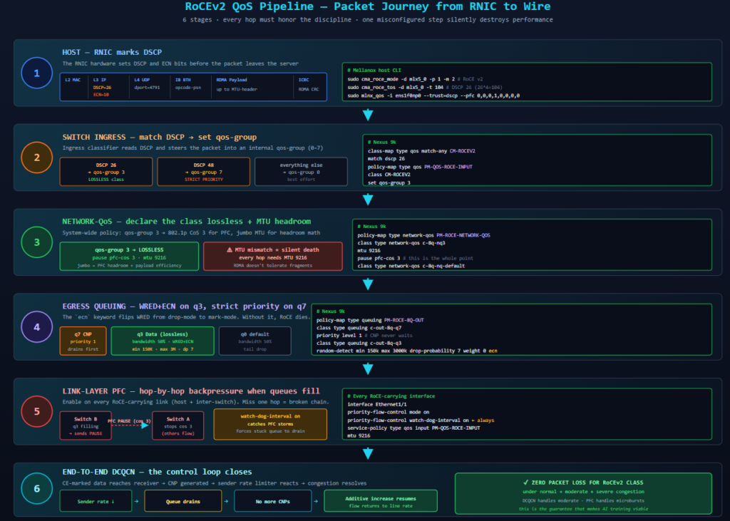
Every step has to be right. Miss the DSCP marking on the host and step 1 fails. Miss the no switchport on the L3 link and step 2 misclassifies. Miss the mtu 9216 on one interface and PFC headroom math breaks. Miss the ecn keyword and WRED drops instead of marking.

RoCEv2 is not “just Ethernet.” It is Ethernet plus a rigorously engineered QoS pipeline. Treat it that way.

---

8. Verification: What to Watch, and What Silently Breaks

The first rule of RoCE troubleshooting: absence of errors is not proof of correctness. You have to look at the right counters.

Command cheat sheet

show policy-map system type qos
show policy-map system type queuing
show policy-map system type network-qos
show policy-map interface Ethernet1/1 type qos
show interface priority-flow-control
show queuing interface Ethernet1/1
show queuing interface Ethernet1/49 | include QOS|drop|ECN|pause
show interface counters errors

Counters that tell the real story

Counter	What it means	If it’s non-zero
Rx Pause per priority	PFC PAUSE received from downstream	Fine at low rate. Sustained = downstream congested
Tx Pause per priority	PFC PAUSE sent to upstream	Sustained = this switch is congested. Investigate
ECN marked per queue	Packets marked with CE bit	Expected on q3 under load. Zero under load = broken
WRED dropped	Packets dropped by WRED (not ECN)	Should be zero for q3 with ECN configured
Output queue drops	Tail drops	Should be zero for lossless class. Ever.
Input errors / CRC	Physical layer	Fix cabling before touching QoS
Interface PFC watchdog shutoff	Watchdog fired	Stuck receiver. Find and fix

The failure modes nobody warns you about

1. MTU mismatch on one hop. Fragmentation for UDP is technically possible, but the RNIC won’t do RDMA over fragmented packets. Symptom: RDMA connection establishes, throughput is a fraction of expected, no obvious error. Fix: show interface | include MTU on every hop.
2. DSCP remarked by a middle switch. A transit device trusting CoS 0 will wipe your DSCP. Symptom: end-to-end classification looks right at endpoints, but PFC counters on middle switches show no activity on priority 3. Fix: show run interface on every hop, verify trust boundaries.
3. ECN not honored end-to-end. If any hop has WRED without the ecn keyword, that hop drops instead of marks. Symptom: RDMA retransmits under moderate load, DCQCN never engages. Fix: show policy-map interface | include ecn on every hop.
4. PFC storm from a stuck NIC. A firmware bug or stuck queue on one host causes it to send PAUSE forever. Symptom: entire rail’s throughput collapses. Fix: watchdog catches it; then RMA the NIC or reboot the host.
5. ECMP hash polarization. All your GPU-to-GPU flows hash to the same uplink because the src port entropy from the RNIC is not sufficiently random. Symptom: one uplink at 100%, others at 0%. Fix: check RNIC firmware for QP hash randomization; verify switch’s hash seed differs between leaf and spine.
6. Buffer allocation too small for headroom. Nexus lets you tune shared buffer per class. Undersized headroom for PFC means the pause frame arrives too late. Symptom: sporadic drops on lossless class under bursts. Fix: show hardware internal buffer info and adjust hardware qos ns-buffer-profile.

---

9. Design Trade-offs and Where to Go Next

If you take one thing away from this post: AI fabric design is a discipline of matching physics to topology to protocol. Every choice cascades.

• Choose 4 nodes/rack because 40 kW/rack is the ceiling.
• Centralize leaves because 256 fibers into one network rack beats 32 fibers × 8 racks with fragmented ports.
• Choose RoCEv2 over IB when your team is Ethernet-native and you want multi-vendor leverage; choose IB when the workload is dense collective-heavy training and SHARP pays for itself.
• Configure PFC because DCQCN can fail. Configure DCQCN because relying on PFC destroys throughput.
• Verify with counters because misconfigurations do not throw errors — they degrade performance until someone notices the training loss is diverging.

The rabbit hole goes deeper. Topics worth their own posts:

• Adaptive routing and DLB (Dynamic Load Balancing) on Broadcom Tomahawk 4/5 and Cisco Silicon One — how to avoid ECMP hash polarization at scale
• Zero-touch RoCE with EVPN-VXLAN overlays — RoCE across a segmented fabric without breaking lossless guarantees
• NCCL topology awareness — how the collective library discovers and uses the physical topology
• Front-end (storage/checkpoint) fabric design — a separate discussion, usually a separate physical fabric
• BGP EVPN + IRB on the front-end, with careful decoupling from the back-end
• Telemetry: streaming buffer occupancy via gNMI/gRPC for real-time congestion visibility
• Power/thermal-aware scheduling — the network engineer’s involvement in workload placement

---

10. Closing

Traditional data center networks are optimized for a mixed, unpredictable workload. AI backend networks are optimized for a single, brutal, synchronous one. The design principles are different, the failure modes are different, and the operational discipline is different.

But the underlying skills — L1 rigor, L2/L3 protocol understanding, QoS discipline, buffer math, systematic troubleshooting — are exactly what a CCIE-trained network engineer already has. You are not learning a new field. You are applying an old field to a new set of constraints.

If you got this far, the next step is a lab. Pull two Nexus 9300s (or Arista 7060s, or an emulator like Cisco Modeling Labs), spin up two Linux hosts with ConnectX-6 or later cards, and run the config in Section 6. Load ib_write_bw and watch the counters. That’s where the real learning starts.